


Airlines have very powerful IT tools to do this. For example, Air France had a specific router tool called OCTAVE, which, based on weather data renewed twice a day and covering the entire world and all altitudes, determined the most economical route depending on the weather of course, but also taking into account other elements such as the amount of overflight taxes, for example, which can vary very significantly from one country to another, and not always in proportion to the service provided…!
For example, this is what the document that was provided to the crew looks like for a flight between Paris and Tokyo, with a B777-200.
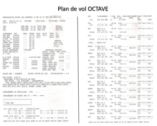
On the left, the first page of the operational flight plan was notably used, during flight preparation, to determine the quantity of fuel to be loaded, and on the right, the first page of the flight follow-up, which was the working document crews during the flight.
The system also automatically developed and sent the ATC flight plan to the air navigation control services.
For reasons of cost reduction, Air France abandoned this “in-house” system and now uses the services of another flight plan provider, LIDO, which I believe is a subsidiary of the German airline Lufthansa.
Other providers such as Jeppesen or SITA (manager of the aeronautical communications system) also provide this type of service, but all this is paid, of course, and is not accessible to the average simmer wanting to make a long-haul flight on your favorite network, even if certain websites or software offer very credible simulations, we will see it below…
Before the massive arrival of computers, as we saw in the NAVIGATION 1 article, all this was done by hand: it was a real job to determine the RTM Minimum Time Route!
We can still do it of course but, with the help of home computing and some basic knowledge, it is now possible to simplify the task a little: this is the summary that we will try to make here .
THE ORTHODROMIC ROUTE
The calculation
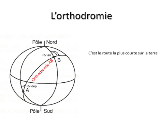
We saw it in the first article NAVIGATION 1, the most direct route on the earth, equivalent on the terrestrial sphere to the straight line on a plane, is in fact an arc of a great circle centered on the center of the earth, which we call an orthodromy.
The disadvantage is that it is not very easy to define its precise characteristics. No navigation map allows it to be traced precisely by drawing a line with a ruler, it is only possible to trace a mapline not too far away. Furthermore, it is not possible, except in special cases such as the equator and the meridians, to follow it at a constant course.
On the other hand, for a moderately powerful calculator, a scientific calculator for example, it is easy to calculate its basic characteristics, that is to say the great circle distance, the true departure route and the true arrival route. This is what INS or FMS navigation systems do, which can only follow great circles.
All these calculations are based on some spherical trigonometry formulas. For math enthusiasts who are interested, here are the three fundamental formulas which allow calculations to be made in any spherical triangle.

For the application of these formulas to navigation, you can refer to the website of a professor from the ENSM (Ecole Nationale Supérieure Maritime) at the following address: http://traitedemanoeuvre.fr/prog_nav_O13.swf.
Several other sites also provide a means of directly calculating the characteristics of the orthodromies, but be careful, some give erroneous results, particularly on the Rv departure which requires a somewhat delicate interpretation!
The route
Let’s return to our practical example, our flight between Paris and Montreal. The first thing to do, to get an idea of the shortest route, is to calculate the elements of the great circle that joins the two airports.
Using a small home-made EXCEL spreadsheet, we find the following elements:
Ortho distance = 2980.5 Nm, Rv departure = 297°, Rv arrival = 237°
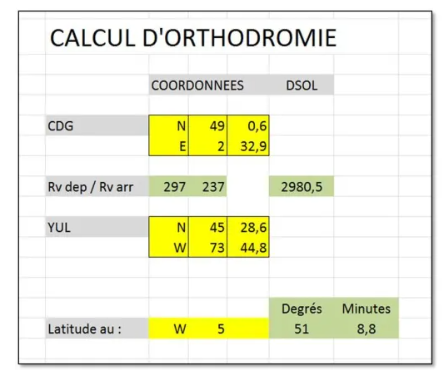
While the latitude of Montreal is lower than that of Paris by approximately 3.5°, we see that the true route Rv from the great circle is 297°, that is to say that it points towards the northwest, towards the south of Ireland!
The lower part of the Excel sheet allows you to mark out the great circle route by calculating the latitude of this great circle route at different longitudes. And we find the following values:
- 51° 09' N at 05° W52° 13' N at 10° W53° 01' N at 15° W53° 36' N at 20° W54° 07' N at 30° W53° 47' N at 40° W52° 36' N at 50° W50° 26' N at 60° W47° 06' N at 70° W
The northernmost point of this great circle, called the VERTEX, is located around point 54°N / 30°W.
The comparison with the rhumb line, with constant true course Rv therefore, is not the simplest because it is difficult to calculate. You can download at this address, http://www.nauticalalmanac.it/fr/pd-fra-navigation.html, an EXCEL sheet which carries out the calculations.
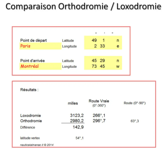
We see that the loxodromic distance would be 3123.2 Nm, which is therefore 143 Nm more than following the orthodromic. This is therefore not negligible since it represents between two and three tonnes of fuel for a B747-400!
And the constant true course of 266° would take us towards Brest…
We can now trace this great circle on a navigation map. The one shown here is the AT 1H ocean hauler from LIDO, which is used for crossings of the North Atlantic.
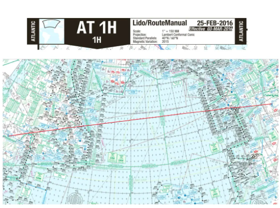
It is, as indicated in the title block, a secant LAMBERT canvas admitting 40°N and 60°N as standard parallels, which makes a tangency parallel equivalent to 50°N. Our orthodromy being located at slightly higher mid-latitudes, the route is practically rectilinear, although with a slight curvature towards the north.
We can therefore remember that on this type of map, if we do not have a means of calculating the elements of the orthodromy as we have just done, by drawing a straight line on the map we obtain a map line which is very close.
Regulatory constraints
To make an oceanic flight plan, you must respect certain rules specific to the airspaces concerned. You have certainly heard of the MNPS zone in particular, which covers a large part of the Atlantic Ocean, in the Shanwick, Gander, Iceland, Santa Maria and New York FIRs. In this zone, the choice of route is free, but it must be divided into segments connecting meridians spaced every 10° of longitude and passing through round values of latitude. In addition, entry and exit from the MNPS zone must be done via anchor points when they are nearby.
For our orthodromic route from Paris CDG to Montreal YUL, the entry anchor point closest to our orthodromic route will be the MALOT point (53°N/015°W), which is located on the edge of the Shannon FIR, in Ireland.
Our flight plan route could therefore begin, after a SID to EVX, as follows:
EVX UT300 SENLO UN502 JSY UN160 NAKID UN80 ARKIL MALOT
Then, we must therefore choose the entire latitude positions closest to the points marking our great circle, which will give:
MALOT 53N020W 54N030W 54N040W 53N050W PELTU
All that remains is to define the domestic route, on the American continent, which gives us:
HAIR YNA J553 YYY J560 YRI OMBRE PAINT
It all ends with an OMBRE 4 arrival in Montreal Pierre Trudeau, CYUL.
This route successively crosses 10 FIRs: on the domestic part first, Paris, Brest, London and Shannon, then the oceanic FIRs of Shanwick until crossing the 30°W meridian, and Gander Oceanic as far as PELTU.
Finally, the domestic route to Montreal takes us through the FIRs of Gander, Moncton, Boston in the USA and finally Montreal.
All these regulatory constraints will certainly lengthen the road, but by how much, it is very difficult to know. To do this, it would be necessary to record the European and American domestic routes segment by segment, calculate each oceanic section with the tool seen above, and add up the total: a hell of a job ahead, with a great risk of error!!! However, this is how flight preparation agents did before the arrival of computer tools! And for the oceanic segments, they had calculation charts which were also available to the crew, on board the plane, to be able to check or recalculate everything in the event of a change of route...
OPERATIONAL FLIGHT PLAN
The operational flight plan is the summary document which will be used to determine the quantity of fuel to be carried on board and to program the navigation systems before the departure of the flight. It is he who will also be used to control navigation and monitor fuel consumption during the flight.
The fuel aspect will be studied later, in a future article…
As we saw in the preamble, to develop operational flight plans, operators today use powerful computer systems. Fortunately for air simulation enthusiasts, there are now websites or software that allow us to develop completely credible flight plans for long-haul flights aboard our simulators.
Among the proposals that I was able to test, I have a preference for the site simbrief.com, and this for several reasons: firstly it is free, which demonstrates a certain generosity on the part of the designers! Then, it allows you to edit flight plans in different formats, including those used by airlines. We are therefore very close to reality.
Simbrief.com offers the Air France format, a true copy of the OCTAVE flight plan, written in French. But there were several formats adapted to different types of flight: the model reproduced by simbrief.com is the one used for medium-haul flights: the navigation log part is not detailed enough to control the navigation of a transoceanic flight. And then it is no longer in service...
It is therefore the LIDO version which will be used in the remainder of this presentation.
The major flaw of simbrief.com is that it does not build the route itself: you must insert the route that you have determined or choose from the last routes that have been used. It will only check its validity against its database. This defect is about to be repaired since, in its latest development, still being tested, it is possible to use Route Finder directly from simbrief. We will experiment with it further…
After having selected the DISPATCH section and created a new flight, let's insert our CDG-YUL great circle route, adjusted to regulatory constraints, as we have just defined it above.
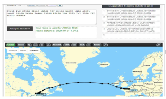
By clicking on “Route Analysis”, we see that this route is correct with respect to the Navigraph 1605 database. And the system tells us that the total length of this route is 3020 Nm. The mention (+ 1.3% ) means that it is longer than the great circle by 1.3%.
We estimated the latter at 2980.5 Nm: 2980.5 x 1.013 = 3019.2. So we are in complete agreement!
The constraints of air traffic rules will therefore impose on us, for this journey, a minimum lengthening of 40 Nm, or 5 minutes of flight and approximately a ton of fuel for a B747!!!
The cartographic representation of the road is, of course, only schematic.
By clicking on “Generate OFP”, the Operational Flight Plan is created according to the criteria that have been selected. You can then view it on screen or make a .pdf file that you can print. As in real life, it can have many pages. The majority is devoted to Notam (Notice To AirMen), which is frankly not essential in the context of our simulated flights...
Here is an overview of the first page which presents the summary of the preparation:
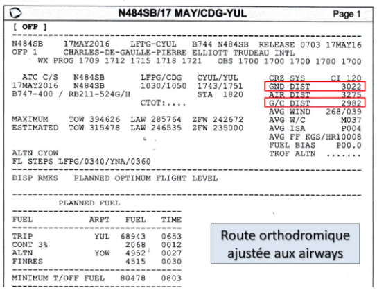
At the top of the page we find a summary description of the flight, and further down on the right (boxed in red), we can read the total ground distance GND DIST = 3022 Nm and the great circle distance G/C DIST = 2982 Nm (Great Circle) . This is very slightly higher than what we found??? Maybe the rounding unless, as real flight plan systems do, the calculation takes into account the fact that the earth is not really a sphere: that would really be the best!!!
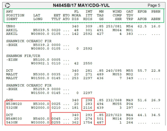
From page 4, we find the navigation log which has the number of pages necessary to describe the entire route. Here is an extract from page 5 for our great circle route to Montreal:
To use this type of document properly, it is imperative to know how to decode it, and this is not necessarily very easy…
Let's first examine the box at the top of each page (here framed in green), filled with various acronyms meant to explain what is found in each of the columns below. Starting from the left, we find successively:
- AWY, POSITION, IDENT: name of the airway if there is one, name of the point and its identification: this is the 5-character code which is used in flight plans and FMS.LAT, LONG: Latitude and longitude of the point.EET, TTLT: Estimated Enroute Time or estimated travel time of the segment, Total Time or total flight time since departure.ETO, ATO: Estimated Time Over and Actual Time Over, the estimated passage times and actual values which will be entered by the crew during the flight.FL, MORA, DIS: Flight Level, Minimum Off Route Altitude, Distance: this is the length of the segment between the two points.IMT, ITT, RDIS: Initial Magnetic Track or Magnetic Route Departure, Initial True Track or True Route Departure, Remaining Distance or remaining distance to destination.MN, TAS, GS: Mach Number, True Air Speed or own speed, Ground Speed or ground speed.WIND, COMP, SHR: forecast wind, component or effective wind, Shear Rate: this is an evaluation of the vertical wind gradient at altitude intended to predict a risk of turbulence. The larger the number, the higher the risk…OAT, TDV, TRP: Outside Air Temperature, Temperature Deviation from the standard temperature, tropopause level.EFOB, AFOB: Estimated Fuel On Board and Actual Fuel On Board: as for the passage times, this is to be completed by the crew while monitoring the flight.PBRN, ABRN: Predicted Burn and Actual Burn?? I haven't found the exact decoding but it is the fuel consumed since departure, the actual amount being noted by the crew.
All these acronyms and others can be found in the HELP section of the site.
Next, you need to clearly visualize how the information is distributed. Take for example the segment between the points 53°N/20°W and 54°N/30°W. It should be noted, first of all, that they are identified by the waypoint codes 5320N and 5430N, a coding that can be used both in flight plans and to insert the route into an FMS. Right next to it, we find their geographic coordinates such that we could insert them to create a new waypoint.
The route information at the start of the segment, Rm and Rv start, are on the same line as the starting point.
Information about the segment itself, distance, mach, TAS, GS, travel time, can be found on the finish point line...
In our example, for the segment going from point 5320N to point 5430N, we can read:
- Rm departure = 298°Rv departure = 283°Distance remaining to be covered from 53N/20W to destination = 2116 NmThe leg will be covered at FL340, at M0.85, TAS = 501 kt, GS = 487 ktThe distance between the two points is 362 Nm, it will take 45 minutes to cover it at FL340At 54N/30W the flight time from the start will be 2h55The wind on the leg will be 229° for 23 kt which makes an effective wind of -14 kt (from face)Etc…
This provision may seem a little confusing at a time when computers make it possible to create documents that are much easier to read. The reason is that, in most companies, these operational flight plans are carried out by specialized services located at the operators' main base, and are then sent to stopovers around the world to be handed over to the crews. Local means are diverse and varied, and possible breakdowns and their more or less efficient means of replacement must be anticipated. They are therefore established in a minimalist format which will allow their transmission by different means ranging from data link to simple telex and their printing by any type of printer.
In addition, they must be able to be transmitted directly to the aircraft, by the ACARS system, particularly when there is a change of route. However, on-board printers are closer to old needle models than to color graphics printers…
Now that we know how to precisely define the shortest route and establish the corresponding operational flight plan, it is time to take into account the actual weather conditions, including wind and temperature...
WEATHER ON THE ROUTE
The theory
Among the weather phenomena which will significantly influence the choice of our route there is the wind, of course, which it is always preferable to have at your back, it's like on a bike!!!
Before studying our concrete case, let's first look at some theoretical concepts that will allow us to properly use weather maps.
In the thickness of our atmosphere, we can distinguish several successive layers which each have their properties. Airliners most often fly in the first, the troposphere, but can also operate in the second, the stratosphere.
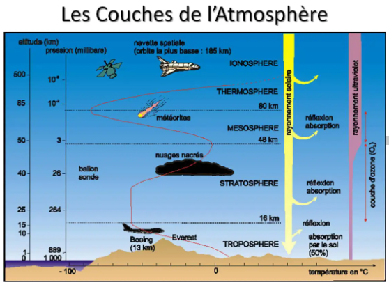
In the troposphere, the temperature decreases as altitude increases (red curve). In the stratosphere, it first observes a plateau before increasing with altitude. It is therefore very interesting to know the limit between the two, called the tropopause.
At the international level, a standard atmosphere has been defined (International Standard Atmosphere ISA), the tables below give an overview of its characteristics.
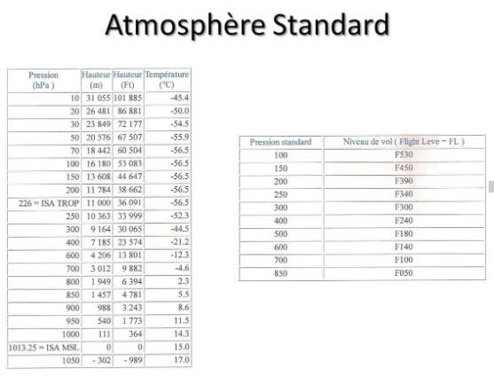
We see, for example, that the standard tropopause is located at 11,000 meters, or FL361, and that the temperature there is -56.5° C.
It is used, in particular, to calibrate an altimeter, which is in fact just a barometer which indicates the altitude corresponding to the pressure it measures. It is also used to determine the deviation from the actual temperature, which is called Δ ISA, and which is used to calculate certain flight parameters.
But, nature being particularly difficult to put into an equation, the real atmosphere never conforms to this model!
In fact, we distinguish three large atmospheric zones which are, starting from the pole towards the equator, the polar, tropical and equatorial air masses.
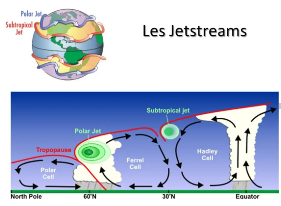
As seen in this diagram, each cell has its own characteristics, notably altitude and tropopause temperature:
- Polar cell, low and warm tropopauseEquatorial cell, high and cold tropopauseTropical cell with intermediate values
Strong wind currents, called jetstreams or more commonly jets, will be created at the break of the different tropopauses. We will therefore find to the north the polar jet, which will be located between FL300 and FL330, and which will undulate like the disturbances of the polar front that it flies over. Further south, we will find the subtropical jet, more stable in direction, and which will evolve around FL390. These two jets generally blow from west to east, but their direction can vary very significantly in places.
This whole beautiful system will evolve in latitude following the path of the sun during the year, and the same two jets also exist, of course, in the southern hemisphere.
And to further complicate all this, we also encounter, around the equator, a pseudo-equatorial jet located at the level of the local tropopause and therefore very high, and which has the particularity of blowing in the opposite direction to the other two, it that is to say from east to west!!!
The jets are, in the northern hemisphere, stronger in winter. Their speed gradient is more pronounced to the north and above, areas which are particularly conducive to CAT (Clear Air Turbulence).
And it is, of course, the opposite in the southern hemisphere.
As one can imagine, Mother Nature will not conform to this simplified theoretical model, far from it, but it is useful to remember this when studying weather maps.
Weather maps
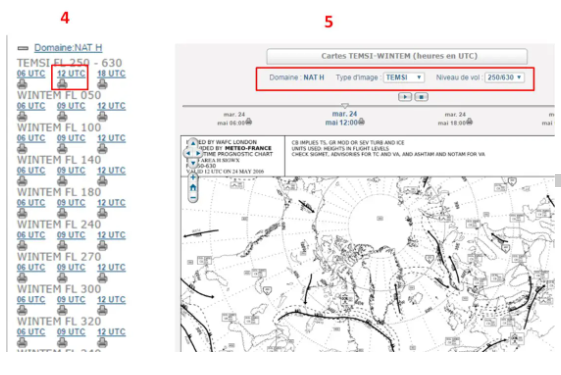
But actually, how do you find these famous cards? The Météo France site specializing in aviation, AEROWEB, is the easiest to use. Anyone can access it, just create their username and password.
The home page is more general aviation oriented. For long-haul flights, you must follow a specific route.
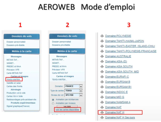
In the left column click on TEMSI-WINTEM… In the new window that opens you must select “View available maps”. For our example, we must then select the NAT H Domain which concerns the North Atlantic.
The list of available cards then appears.
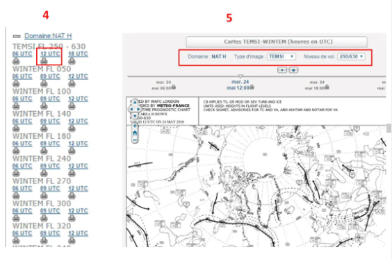
Just select one and then you can change it using the selection windows at the top of the map.
But back to our Paris-Montreal flight. I prepared this article on May 17, 2016. Here, first of all, is an extract from the TEMSI card valid that day at 12:00 UT.
What can you see on a TEMSI card? The SIGNIFICANT WEATHER, that is to say all the weather phenomena affecting the planes which operate in this region and in the range of flight levels indicated in the title block, F250 to F630 for this map, but it is not always the same slice.
We therefore find, among other things:
- A base map, this could be a stereo-polar but this is not always the case Cloud masses, mainly stormy since they exceed FL250 Possible cyclones or tropical storms, as well as volcanic ash clouds Jets with their speed and their altitude The zones of turbulence, icing, etc. The altitude of the tropopause with the low pressure and anticyclonic centers.
We see, from the outset, that the situation is not as simple as in the theoretical diagram... Nevertheless, we can distinguish for example two low pressure centers marked L, one off the coast of Ireland and the other above Newfoundland, where the tropopause is particularly low (FL240 and FL230).
Several jets are indicated: the one circulating across the entire view, at FL320, can be identified as the polar front jet. Its force reaches 140 kt above the great American lakes and around 20°W. The mention 150/430 indicates that its force is greater than 80 kt from FL150 to FL430!
The areas surrounded by dotted lines are those where the presence of turbulence in clear skies is probable, therefore rather to the north of the jet and above.
The subtropical jet is also indicated in places: over the center of the USA at FL380, where it splits into two parallel currents, over Morocco and Algeria, at FL420.
We can also see a stormy area, south of the polar jet, between 40°W and 50°W.
If we follow a route close to the Paris-Montreal great circle, here drawn in red, we will find ourselves confronted with particularly strong headwinds. It will then be in your best interest to choose a route that avoids areas where the wind is strongest. But we will then increase the ground distance! The whole problem, when choosing the route, will be to find the right balance between increasing the ground distance and reducing the headwind...
This time it is the WINTEM card which will be precious to us. We should even say WINTEM cards because, to do it well, it would be necessary to interpolate the values read on several cards, FL320, FL340, FL360 or FL390.
To simplify this presentation a little, we will only use the 250hPa/FL340 here.
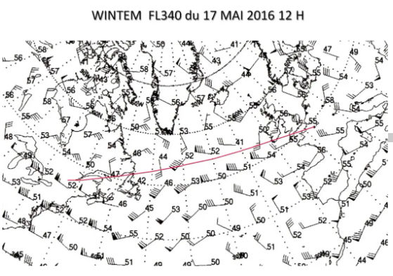
The base map is the same as the TEMSI map. Given the surface area represented, the scale is very large, which means that the density of information is rather low... We will have to be content with that!
This WINTEM map gives the winds and temperatures at FL340. The wind is represented by an arrow indicating the direction in which it blows, the “feathers” of the arrow giving its speed: a line for 10kt, a half line for 5kt, and a triangle for 50kt. Thus, above Montreal, we see that the wind blows from approximately 280° and that its force is 105kt.
The numbers that appear next to it are the temperature values. It is indicated in the title block that these temperatures are always negative unless the sign is mentioned, which would be very surprising at these altitudes!
With the outline of the great circle, in red, we can clearly see that it is in the north that we will find winds that are less strong and oriented in a more favorable manner. It's all about finding the best compromise...
CHOICE OF THE BEST ROUTE
Les tracks
In this region of the Atlantic Ocean, the OTS system (Organized Tracks System) will be able to help us.
Every day, hundreds of planes cross the Atlantic Ocean to connect Europe to North America. The problem is that all companies use aircraft types with comparable characteristics, and wish, for reasons of scheduling convenience and use of their fleet, to fly west during the day and east at night. .
If each plane follows the route of its choice, air traffic control will quickly find itself overwhelmed and unable to manage everything, especially since there is no radar in the middle of the ocean. This is the reason why the services responsible for air traffic control over the North Atlantic publish, every day, preferential routes called North Atlantic Tracks NAT. Their use, in the choice of route, is not obligatory but strongly recommended, especially since the oceanic clearance will, in the track area, practically always be aligned with the nearest track...
The Shanwick control therefore edits the daytime tracks, while the Gander control takes care of the nighttime tracks. They are centered on the average minimum weather route between the two continents established taking into account the day's weather forecasts.
They are designated by a letter of the alphabet, starting with A for the northernmost track in the day system, and with Z for the southernmost track in the night system.
For our flight on May 17, 2016 leaving at 10:30 a.m. Z from Paris CDG, here is an extract from the valid tracks message:
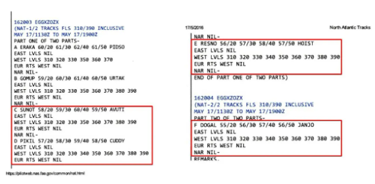
At the top left we read that it was issued by Shanwick, EGGXZOZX, and that the period of use goes from 11:30 a.m. Z to 7:00 p.m. Z, the time of crossing the 30°W meridian.
France being one of the southernmost countries of the countries concerned, it is generally among the last tracks that it will be appropriate to choose the one which will give the best route: we will therefore study tracks F, E, D and C.
Here is what it looks like when plotted on the map:
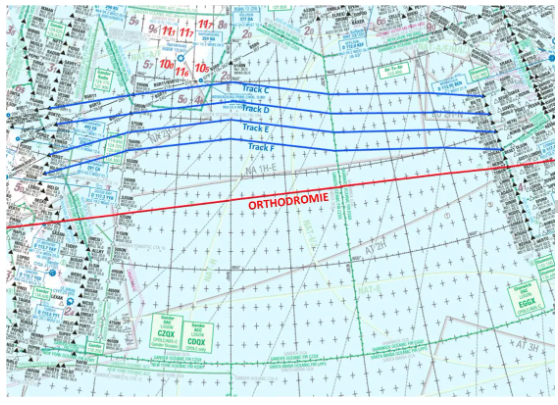
The tracks are spaced by one degree of latitude, i.e. 60 Nm, which complies with the standards of the MNPS space in which this part of the Atlantic Ocean is located.
If we plot these tracks on the WINTEM map seen previously, here is what we obtain:
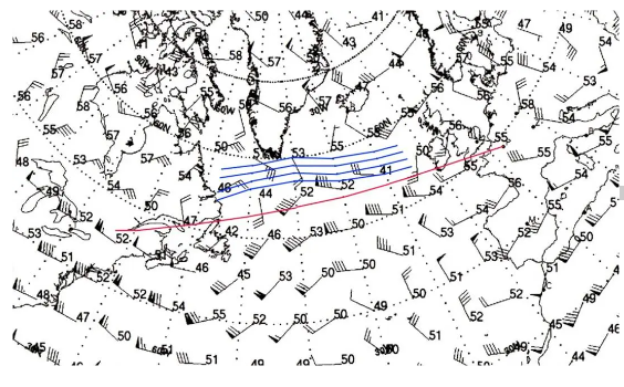
We see that the OTS system has been defined north of the great circle, avoiding the area where the westerly winds are the strongest. We even manage, at the end of the tracks, to have a tailwind component!
It remains to be seen how to determine which will be the best option and which track will give the lowest consumption, because it is in these terms that the problem must be evaluated.
Air Distance
It is very difficult to compare different routes which will be traveled with different ground speeds since wind and temperature will vary. We will address this subject more precisely in a future article devoted to determining the quantity of fuel necessary for a flight.
However, we can say that the temperature has no influence on the distance consumption because it acts in the same proportions on the consumption and the aircraft's TAS speed.
For the wind, to be able to make route comparisons, the simplest thing is to transform the Ground distances into Air distances, which amounts to finding, for the same flight time, what would be the equivalent distance to travel if it were not Was there no wind?
We therefore determine the air distance Da using the formula:
Ds / GS = Da / TAS ou Da = Ds x TAS / GS
The total Air distance of a route will be the sum of the Air distances of each route segment. And it is the lowest total Air distance which will be the criterion defining the best route of the day.
So let's see, for our Paris-Montreal flight, what will be the best choice among the different tracks available that day.
The best route
To begin, let's remember the characteristics of the road closest to the great circle:
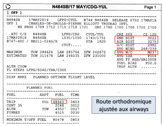
We remember that this route measures 3022 Nm in ground distance, which is already 40 Nm more than the LFPG-CYUL great circle. But if we decide to take this route, taking into account today's weather, we will experience an unfavorable average effective wind of -37 kt (AVG W/C). This will make a total AIR DIST air distance of 3275 Nm and a TRIP FUEL stage load shedding of 68943 kg.
If we decide to take the southernmost track of the OTS system of the day, track F, let's see what that will give:
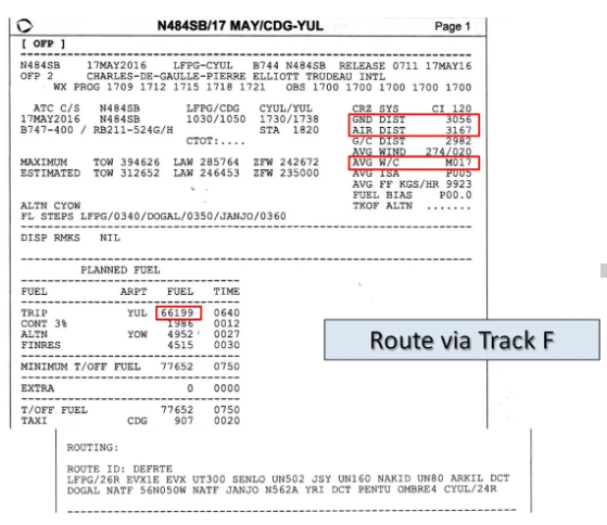
We see that the ground distance is greater, 3056 Nm which is 34 Nm more than the previous one. But the air distance decreases significantly, 3167 Nm for an average effective wind which falls to -17 kt, which therefore represents a significant reduction in the air distance of 108 Nm and a stage load shedding of 66199 kg, a reduction of more than 2.7 tonnes!
Note in passing that the module which gives access to Route Finder is very useful in this case since it knows the tracks of the day and allows you to adjust European and American domestic routes.
We continue our search by choosing track E, one degree of latitude further north:
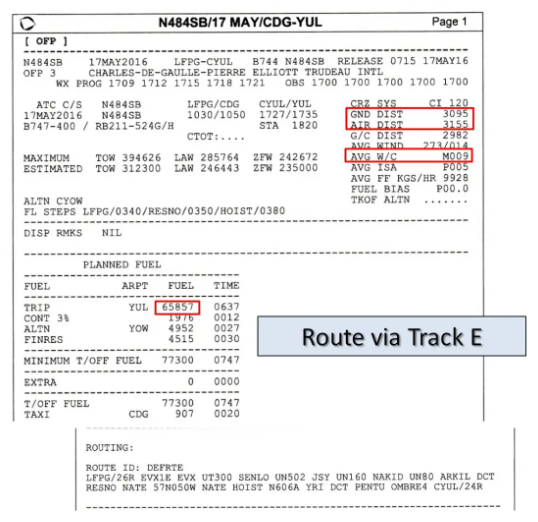
The ground distance increases by another 39 Nm, reaching 3095 Nm, but the air distance, at 3155 Nm, saves another 10 Nm compared to the previous one and the stage load shedding, of 65,857 kg, saves another 342 kg. on track F.
You understand the system, just continue track by track until you find the one from which the increase in ground distance will no longer be compensated by a more favorable air distance.
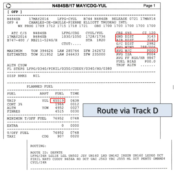
Track D, with its air distance of 3141 Nm and an average effective wind equal to 0, saves us another 14 Nm and 338 kg of fuel...
On the other hand, the route via track C sees its air distance increasing:
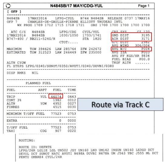
Despite a positive average effective wind of 4 kt, the air distance of 3171 Nm is greater than that of track D because the ground distance has further increased by 52 Nm…
The best option will therefore be the route which takes track D.
We will therefore choose a route which will be 121 Nm longer than the route closest to the great circle, but which will save, thanks to careful consideration of the weather forecasts, more than 3.4 tonnes of fuel. !
It is quite obvious that for an airline which operates several dozen long-haul routes of this type daily, the impact on the annual financial statement will be very significant!!!
The implementation of efficient computer systems and the notable improvement in weather forecasts en route, in particular thanks to satellites, have made it possible to make great progress in this direction.
And at our level of simmer, the arrival of systems like SimBrief.com allows us to also take advantage of it to make our flights as close as possible to reality...
Insertion into the FMS
All that remains is to insert this route into our navigation system. Here is what it looks like in PMDG’s B747-400:
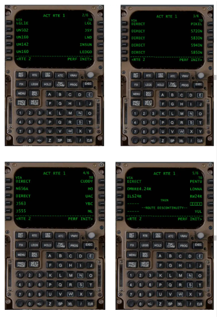
We will need no less than four pages of CDU to insert everything…
Note that I used, for track D, the identifiers of the points as they appear in the navigation log and which we talked about above: 5720N, 5830N, etc… They are known from the database in as waypoints.
But be careful not to make a mistake when positioning the letter N: the consequences would be unfortunate, as we can see in this example...
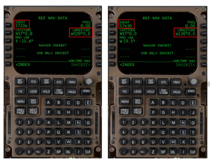
This view allows us to note a small discrepancy in the mode of indication of the magnetic declination, as it usually appears on maps, and the way in which the MAG VAR is indicated in the REF NAV DATA screen of the CDU: for the point 5720N for example, we read E -10.4° while the maps indicate, for this region, a W declination. On the other hand, the sign – conforms to customs and customs, as do the calculations which use it…? ??
You can also insert an oceanic point by creating a new point using its geographic coordinates, but this is only possible on the LEGS page, and it is significantly longer and subject to error...
In all cases, the first thing to do, as soon as you have finished the insertion, is to check the total ground distance and compare it to that indicated in the flight plan. This will be a good indicator to confirm that there was no insertion error…
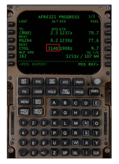
On the PROGRESS 1 page, we see that the FMS has calculated a distance, to CYUL, of 3140 Nm to compare with the 3143 Nm indicated in the flight plan: up to rounding, "the error is correct" as they say often in the cockpits!
It is also good to check the distances between each point, and the magnetic routes starting from each oceanic leg. They can be found in the different LEGS pages available at the CDU.
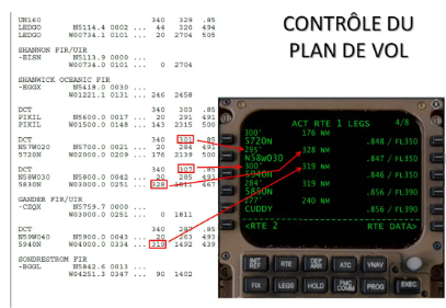
We can note on this screen that the point 58N030W has been inserted by its geographical coordinates as indicated above. It therefore appears differently from those which are inserted with their Waypoint identifier known to the FMS database.
On the distances no problem, however there is a significant difference, 6 to 7°, between the departure Rms indicated by the FMS and that indicated in the flight plan. Who is wrong, who is right?
Let's try to answer by doing the calculations on two sections, the one which goes from 5720N to 5830N and the next which goes from 5830N to 5940N:
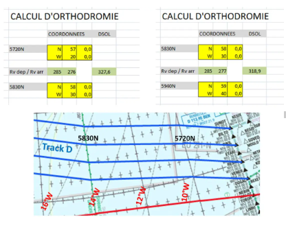
For the distances, no problem, we agree: the first segment is 328 Nm and the second 319 Nm.
For the Rv departures, we are still in agreement: we find Rv = 285° at the start of these two sections when SimBrief finds 284° for the first and 285° for the second. The roundings certainly…
On the other hand, if we note the magnetic variations on the map, we find between 10° and 11°W for point 5720N and 16°W for point 5830N. This therefore gives us a departure Rm of 285 10 = 295° at the departure of 5720N and 285 16 = 301° at the departure of 5830N, that is to say, to one degree, those indicated in the CDU!
It therefore seems that it is the magnetic variations taken into account by SimBrief.com which are incorrect: nobody is perfect!
In a real B744, if you place the NORM/TRUE switch to TRUE, all route and heading indications become real, including CDUs. In the PMDG model, the CDUs remain magnetic which is a shame because we could have verified the true routes calculated by the FMS. You will have to wait until you have completed the flight to check the ND as you pass each point…
CONCLUSION
During this small study, we therefore determined that the best route to go from Paris to Montreal, on May 17, 2016, was the one that took track D of the day. In a future article, we will see how to calculate the quantity of fuel to carry to carry out this type of flight, knowing, of course, that all the study we have just done was aimed at minimizing this carry...
Good flights...!