


As soon as man seeks to travel, whether on foot, on horseback, by car, by boat or by plane, the first problem that arises is to choose the route to follow. Not very complicated if the journey is short, you know the terrain well and you have numerous reference points. The problem becomes more complicated if we want to go very far, cross an ocean or a desert, if it is night or we fly over a cloud layer. This is the whole purpose of navigation, the basics of which we will study here…
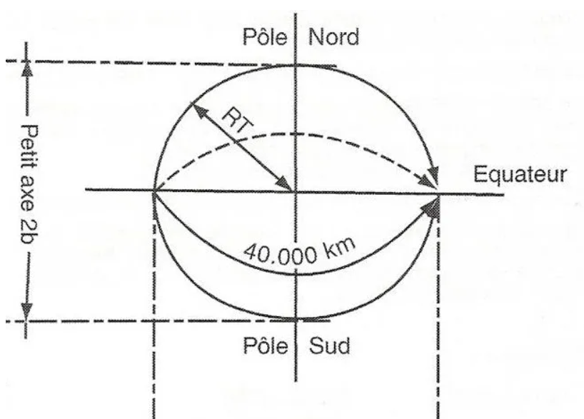
Our earth is an ellipsoid of revolution comparable, to simplify, to a sphere with a mean radius of 6337 km. The difference between the minor axis and the major axis is approximately 22 km, the average perimeter is close to 40,000 km.
The earth rotates on itself, around its North South axis, in 24 hours, and around the sun in 365 days. The axis of the poles is inclined by 23°27' relative to the plane of the ecliptic, which is the origin of the seasons.
To enable positions to be identified, different systems have been designed. The best known and most common is the one which, thanks to the equator, separates the earth into two hemispheres. Parallel to this equator are defined parallels which define the latitude L. It is counted from 0° to 90° towards the North or towards the South.
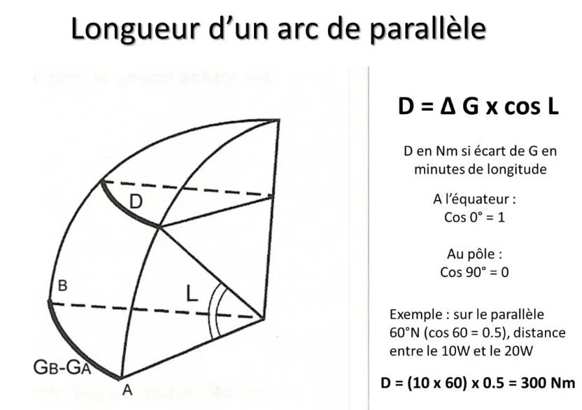
For mathematicians, and without going into a complex mathematical demonstration, by simply remembering that the cosine of the latitude decreases from 1 to 0 when it increases from 0° to 90°, intuitively we will remember that the length of an arc of parallel varies according to the cosine of its latitude…
L’ESTIME (dead reckoning)
This is the basis of all navigation. And this is still relevant today since the most modern means of navigation do nothing more but with the great precision that current technology allows, we will talk about it again when we look at these tools.
Whatever our means of transport, to go to point B from point A, we must start by steering, or directing our vehicle towards point B. This is the most important but it is not necessarily the simplest: let's remember Christopher Columbus heading west to go to India...!
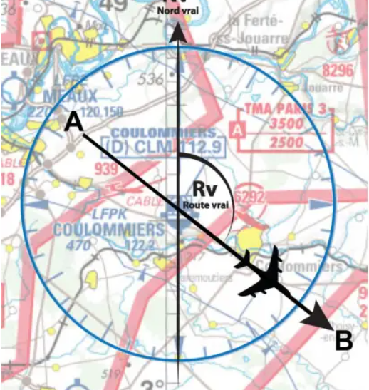
We must therefore be able to say in which direction B is located, and in relation to which reference, generally the direction of the North Pole. This is the true course angle Rv, expressed in degrees relative to Nv, clockwise.
If we see B from A, it's easy but it's rare! We can go from visible point to visible point, this is what we do in visual flight. If this is not possible, or if you want to control navigation visually, you will have to measure it on a map or calculate it...
Then you will need to know the distance to travel to reach point B, or an intermediate point if one has been defined. We can then estimate the flight time to complete this journey by dividing this distance by the speed relative to the ground.
The course angle Rv and the travel time will be the two elements which will allow us to navigate “by dead reckoning”. We also say “head and watch”.
Among the most commonly used means of determining the two elements of dead reckoning, which are course angle and distance, are, of course, maps.
CARTOGRAPHY
Lots of reasons, including navigation, led to wanting to represent the Earth. But it is very difficult to do it faithfully, in particular because of its not very… Catholic form (cf. Galileo and Copernicus)!
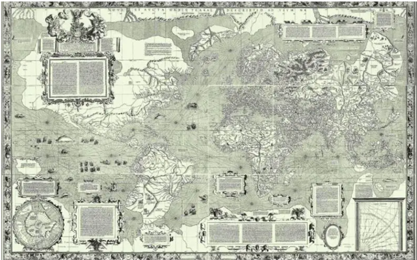
The most faithful representation is the world map: obviously on a very large scale, and really not practical to use on a plane!!!
General
For maps, representing a vaguely spherical object on a flat sheet of paper is not possible with precision: it will therefore be necessary to make compromises, and choose which elements to reproduce faithfully to the detriment of others which will be less faithful or not at all. at all !
For navigation, one of the most important points, as we have just seen, is the orientation of the trajectory with the road angle Rv.
Conformity
We must therefore be able to measure the angles precisely: this is what we call conformity. On a conforming map, if two lines intersect at an angle of 47° on earth, their representations on the map will also intersect at an angle of 47°. The angles are therefore preserved.
For a map to be compliant, the scale around a given point on the map must be constant in all directions, and in particular in the two perpendicular directions that are meridians and parallels.
Why is it so important to measure angles accurately?
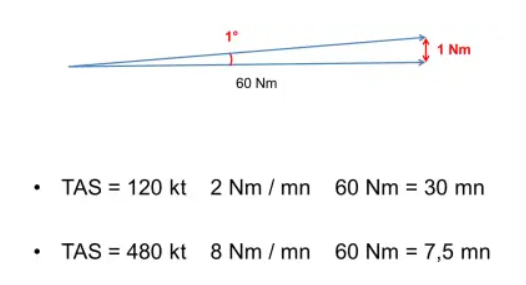
With just one small degree of error, after 60 Nm the deviation is 1 Nm from the road! And 60 Nm is 30 minutes in the C172, but barely 8 minutes for a Jet in cruise! And there are multiple sources of error: measurement, navigation instrument error, wind drift, etc.
The right card
Then, it would be good if by drawing a line on the map with a ruler we defined the trajectory we want to follow, orthodromic, rhumb line or other “dromy”, we will come back to that.
Equidistance
And finally, to measure distances, if the scale was constant throughout the map (we would then say that it is equidistant), that would be perfect! In fact, as we have just seen, this is not a big problem knowing that we can always measure a distance by plotting it on the nearest meridian and counting the minutes of latitude, in other words nautical miles!
Having these three qualities with precision is impossible: the aeronautical charts will therefore first be compliant. For the rest, you will have to choose the most suitable compromise.
AT CARTE MERCATOR
Developed in 1569 by Gerardus Mercator who gave it his name, it is certainly the best-known representation of the world.
Features
It is a cylindrical projection tangent to the equator. However, it is not a geometric projection: the spacing of the parallels is calculated mathematically so that the map is compliant, and therefore usable in navigation (increasing latitudes, primitive of 1/cos L).
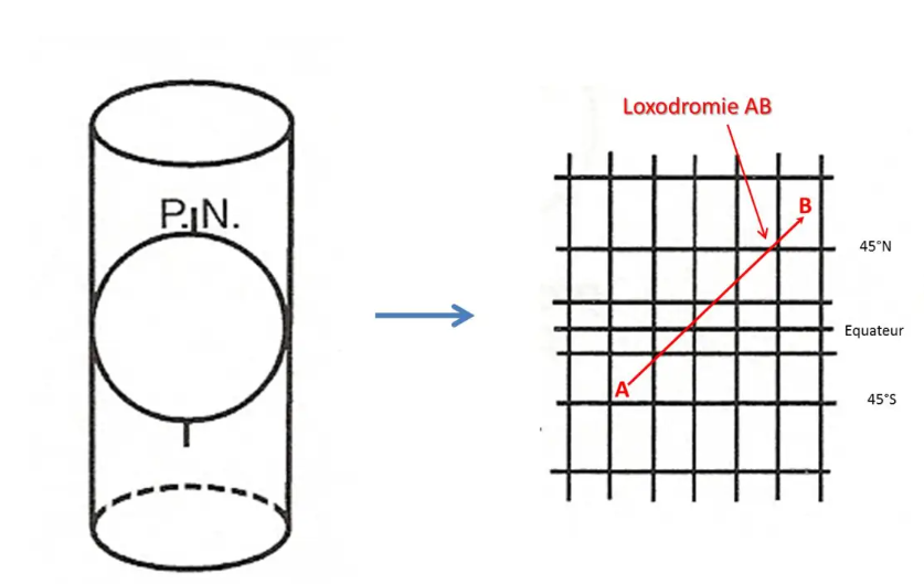
The parallels and meridians are represented by straight lines perpendicular to each other: this is very practical for navigating at a constant heading because if we draw a line on the map, the Rv is the same throughout the route: the route thus traced is called a rhumb line.
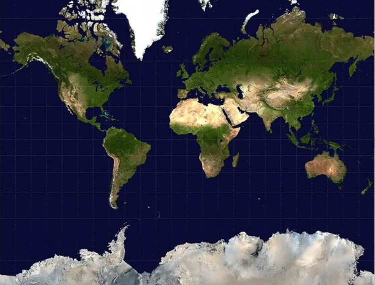
The scale, on the other hand, is very variable, which considerably distorts the surfaces: Greenland, with its 2 million km², seems as vast as the whole of Africa, which is approximately 15 times larger!!!
The scale is minimum at the equator and increases towards the poles.
It is not possible to represent the polar zones on a Mercator map.
The route from Paris to San Francisco shown on the airlines' planispheres makes a beautiful loop over Greenland and Hudson Bay in Canada, while the straight line would pass over New York??? Those who have had the chance to fly to the west coast of the USA can confirm that we are indeed flying over the great North.
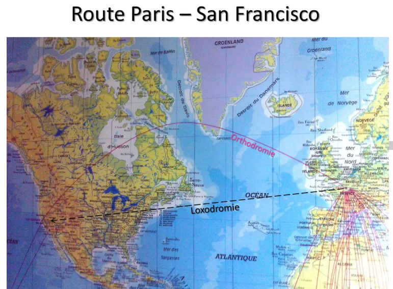
In fact, the rhumb line is not the most direct route: the straight line on our spherical earth is in reality an arc of a great circle (whose center is that of the earth) passing through our two points A and B. For to have confirmation, on a world map, by stretching a wire between Paris and San Francisco we will materialize the shortest route. This is called an orthodromy.
To give you an idea, the great circle distance between CDG and SFO is 4836 Nm while the loxodromic distance is around 5600 Nm: 800 Nm, the difference is not small!!!
Constructing a Mercator map precisely is a matter for professionals: thank you IGN. On the other hand, we can easily construct a small piece of it graphically.
Building a Mercator map
To illustrate this, I offer you a little practical exercise:
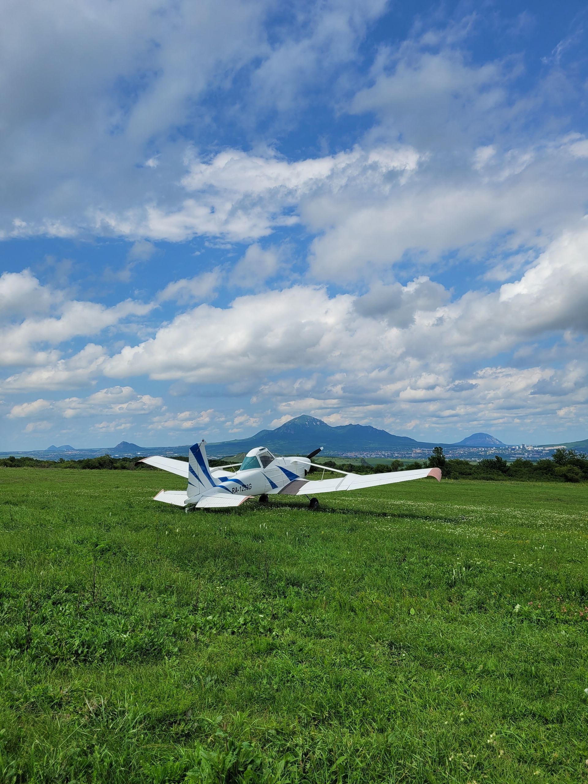
Let's imagine that you inherit from your grandmother a nice sum of money and a large piece of land located in the southwest, around 45°N and 1°30 E. With the money you decide to buy an ultralight aircraft, and with the terrain to make a track to use it… You want to make it the VAC map, both to know the QFU and the length of the track, and also to make it known to other users.
First draw a rectangle 12 cm high and 14 cm wide. The vertical sides will be the meridians, the horizontal the parallels of our Mercator map.
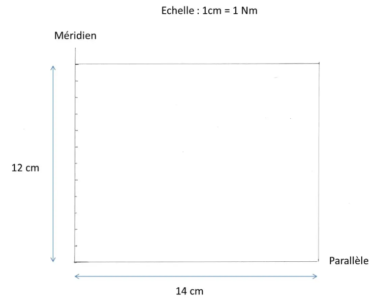
Scale the left vertical side from cm to cm. We will set the scale: 1 cm = 1 Nm.
Draw a line coming from the bottom left corner, and forming an angle of 45°, the latitude of our land, with the bottom parallel. We can also do this by drawing the diagonal of a square…
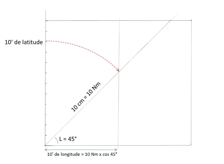
On this line, transfer the 10 cm meridian representing 10 minutes of latitude, therefore 10 Nm. Lower a vertical line onto the bottom parallel. We have just delimited the length of a segment of 10 minutes of longitude: as we saw above, it measures 10 x cos 45° or approximately 7 Nm, therefore 7 cm on our map. (cos 45° = 0.707, like the sinus, the most aerodynamic of the sinuses!!!).
The scale is therefore the same on the meridian and on the parallel: our canvas is therefore consistent!
You understand better why I chose a rectangle 14 cm wide… which therefore represents 20 minutes of longitude.
All that remains is to graduate our longitude scale every 7 mm.
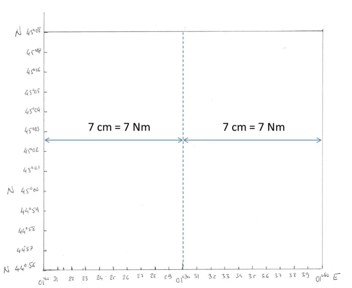
To have our track approximately centered, we will encrypt the latitudes from 44°56' to 45°58'N, and the longitudes from 001°20' to 001°40'E.
We have just created a consistent canvas (same scale on the meridians and parallels). It is a Mercator canvas since the meridians and parallels are perpendicular lines!!!
With your GPS, you went to measure the position of the two QFUs: to the NW: 45°02.6 N and 001°28.3 E and SE 45°02.2 N and 001°29.8 E. All that remains is to position them on our map .
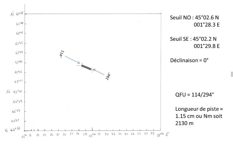
With a protractor you can now measure the QFU, and with a double decimeter the length of the track: I found, for my part, the QFU 114°/294° and a track length of 1.15 cm, therefore 1.15 Nm, or 2130 m.
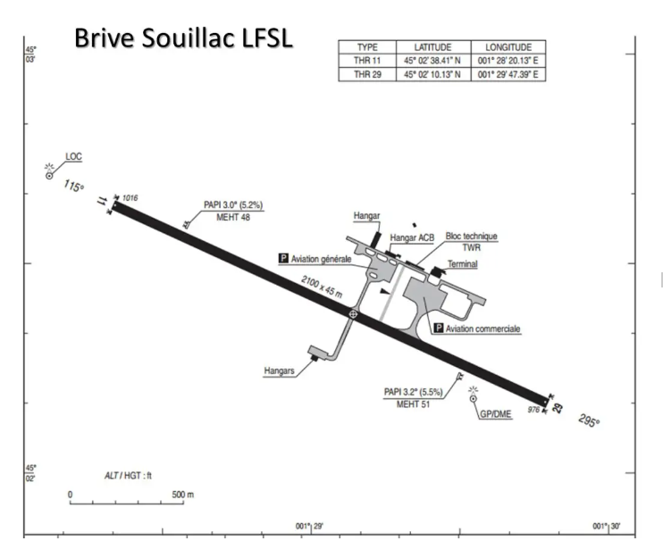
By digging a little into the SIA files, you will easily find that your grandmother has, in fact, left you the land of Brive Souillac, whose QFU are 115°/295° and the runway length is 2100 m!!!
In aeronautics
The Mercator projection is rarely used for aeronautical navigation charts. Only equatorial regions will make it possible to have a map that is both conformal, of course, but also practically orthodromic and equidistant since it is close to the equator.
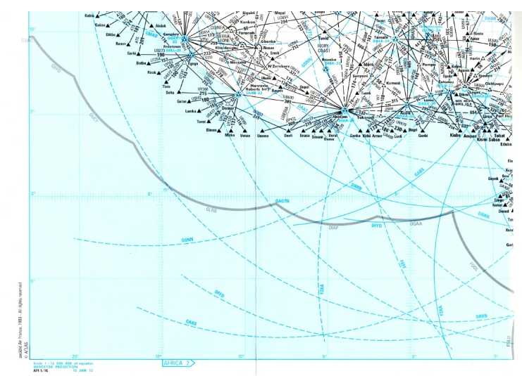
This AFRICA 1 road map for ETOPS flight planning is one of them, although it is not really a navigation map (click to enlarge).
THE LAMBERT CARD
One of the major flaws of the Mercator map is that the straight line on the map does not represent the straight line on earth. But solutions exist… the first is called the Lambert card.
Features
Presented at the end of the 18th century by the Alsatian mathematician Johann Henrich Lambert, it is a conformal conic projection which tangents the terrestrial sphere along a parallel. As with the Mercator map, it is not a geometric projection but a mathematical construction.
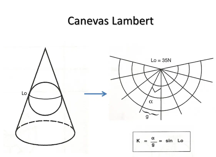
The meridians are represented by straight lines which converge towards the pole. We call the convergence factor K the ratio between the angle formed by two meridians on the map and the angle they form on earth. If the parallel of tangency is of latitude Lo, the factor K = sin Lo.
Parallels are represented by concentric circles.
Like all conformal maps, this type of map is practically orthodromic near the tangency parallel, that is to say that the straight map is practically the representation of an orthodromic. The Mercator map is, in fact, a special case of the Lambert map where the tangency parallel is the equator! It will therefore be orthodromic close to the equator.
To have a Lambert orthodromic map it will therefore suffice to choose a tangency parallel centered on the area that you wish to represent…
As with the Mercator map, the scale is minimal at the tangency parallel Lo and increases significantly as we move away from it.
To remedy this drawback, so-called “secant” Lambert conic maps were created. The official scale of the map is only real at the level of two parallels located on either side of the parallel of tangency. This amounts to saying that the projection cone cuts the surface of the earth along these two so-called “standard” or “conserved scale” parallels. The scale is slightly smaller between these two parallels and a little larger beyond, which gives a practically equidistant canvas over a larger area!
The factor K is then the sine of the mean latitude between the two standard parallels, or approximately because the variation in scale is not symmetrical on either side of the parallel of tangency.
Most aeronautical charts used in our mid-latitude regions are of this type. Thus we can read on the VFR map at 1:500,000 of north-west France published by the IGN: “Lambert conformal conic projection. Parallels of preserved scale 45°54' and 47°42'" (the standard parallels).
This makes a mean latitude Lo = 46°48' N and therefore a factor K = 0.728.
In aeronautics
Here, for example, is an extract from the ATLAS 55C truck used for North Atlantic crossings (here a Paris-New York flight), and whose standard parallels are 37° and 65° N (click to enlarge).
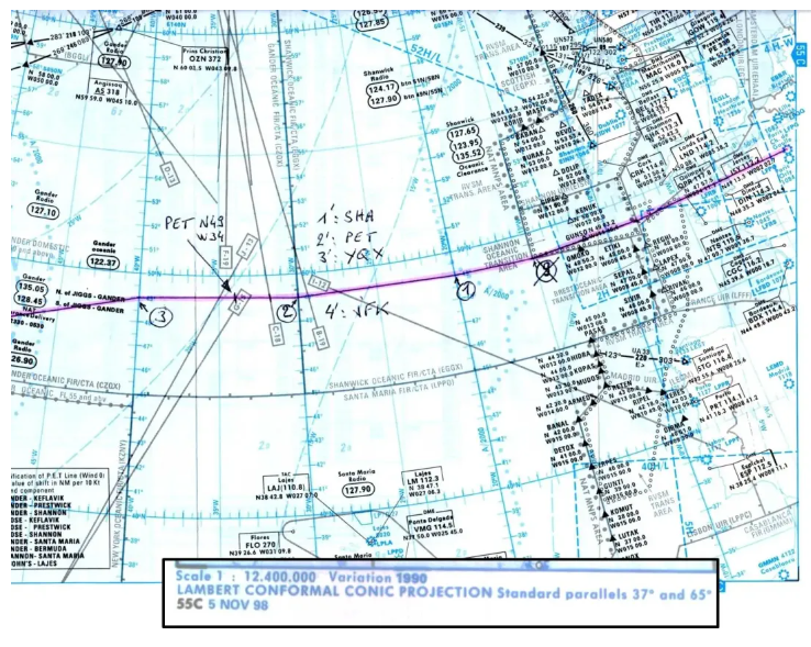
We can clearly see the meridians, represented by straight lines, which converge towards the North Pole, and the parallels which are represented by concentric circles.
With this type of map we are very close to the perfect map: in the area represented, it is consistent for precisely measuring routes or bearings, orthodromic for tracing the shortest routes with a ruler, and practically equidistant since the scale varies little: the holy grail of the cartographer!
Curiously, the SIA "En route" map, although not indicated, is a Mercator map, which is easily verifiable with its parallel meridians, while it presents airways defined by VOR radials, which are orthodromia???
*
What type of card?
To close this chapter: let's try to determine what type of canvas is used by the SIA to present the SIDs and STARs: let's take for example one of the LFPG SID cards.
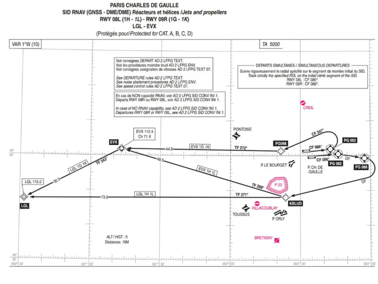
With a ruler or by approaching a parallel to the edge of the screen, we see that the parallels represented are not straight lines. And by measuring the distance between two meridians at the top and bottom we see that they are not parallel.
It is therefore not a Mercator canvas, certainly Lambert, but the small size of the piece represented does not allow measuring the angle between two meridians which would have to be compared to their longitude difference to determine the factor K and therefore the parallel of tangency…
For more information on Lambert cards used in France, you can refer to the Wikipedia page on Lambert cards:
https://fr.wikipedia.org/wiki/Projection_conique_conforme_de_Lambert
OTHER TYPES OF CARD
With the Mercator map for the equator region, and the Lambert map for the other latitudes we solved almost all the problems. There remain a few special cases which gave rise to the invention of (very) particular cards.
The polar stereographic map
The first of these cases is a map made to represent the polar regions: this is called the polar stereographic canvas. It is a projection onto a plane tangent to the pole. And this time, we could really construct it by geometric projection from the opposite pole.
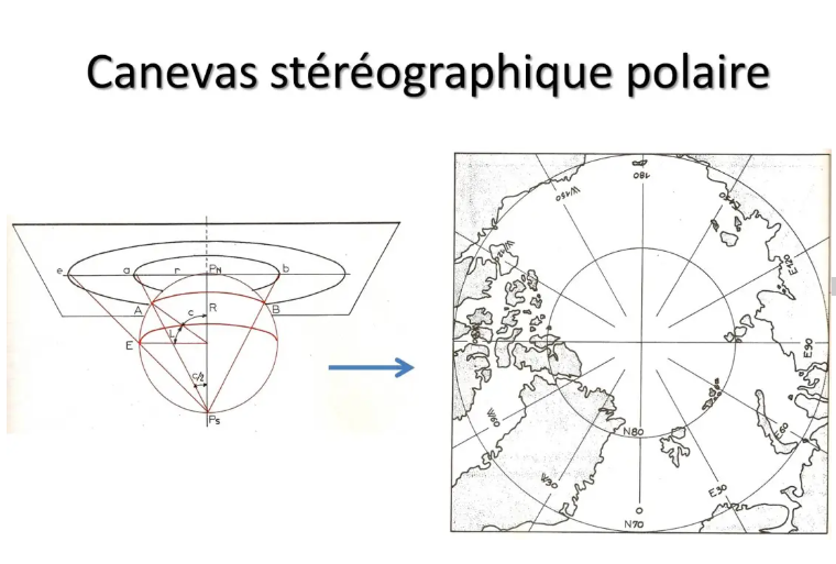
This gives us a map where all the meridians are represented by straight lines starting from the pole in the form of a 360° rose. Parallels are concentric circles.
This map is, of course, compliant to be used for navigation. It is orthodromic near its point of tangency, the pole.
The scale will be minimal at the pole, and will increase away from you.
Its use is therefore limited to the representation of polar regions and associated routes. Here is an extract from the ATLAS 90C polar roader:
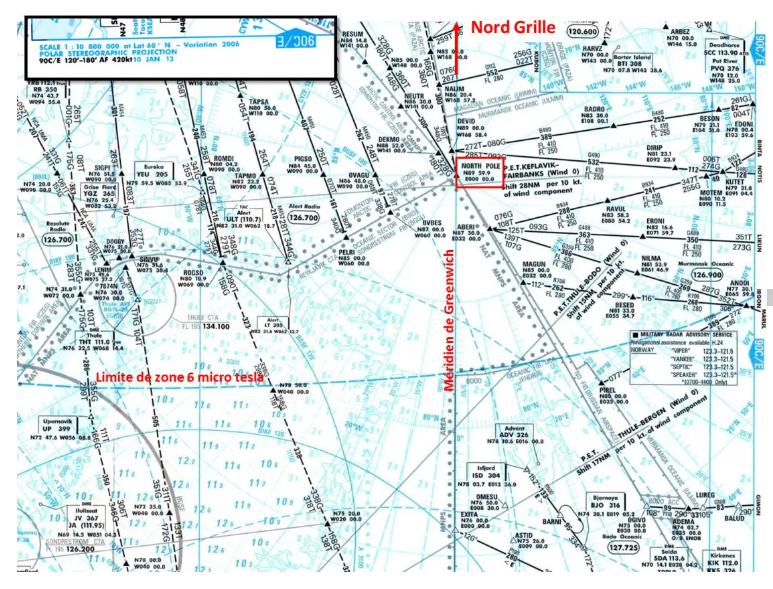
The very strong convergence of the meridians and the unreliability of magnetic compasses in the polar regions (zone 6 micro teslas) make it very difficult to follow a route at a constant heading. For this, the map has a grid oriented following a North Grid to navigate at a constant Route Grid Rg.
Other types of canvas have been imagined and used in the past.
The Transverse Mercator map
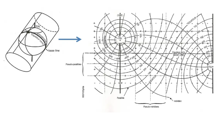
Based on the idea that the equator is a large circle, so-called transverse Mercator maps were designed on the same principle as the direct Mercator, a cylindrical projection, but having as "equator" the Greenwich meridian and the meridian 180° (we can also do it according to any meridian pair and its antimeridian).
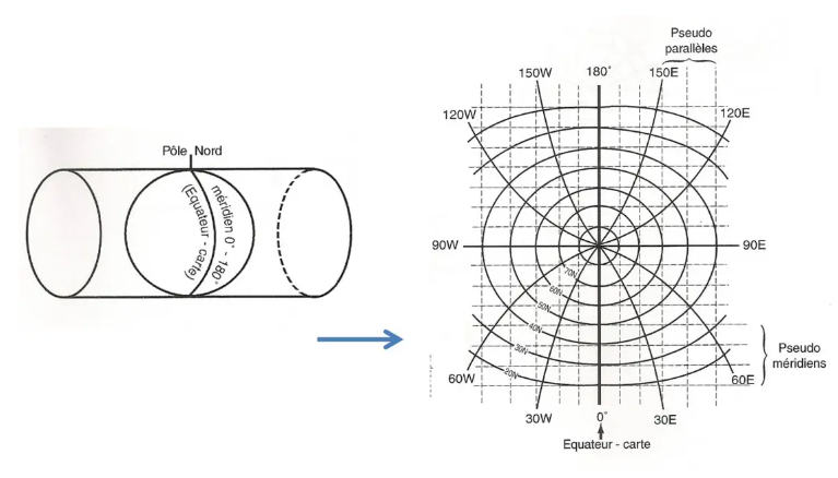
This gives a canvas which will be conformal, of course, and orthodromic on each side of its map equator, which will also be the only one to be represented by a straight line. It is therefore imperative to use a grid with “pseudo parallels” and “pseudo meridians”…
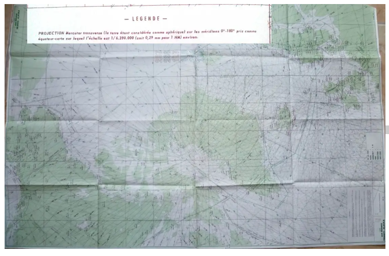
It was on this model that the Air France “France-Alaska” map was made, used before the arrival of INS inertial navigation systems and during the Cold War, a period during which flying over Siberia was prohibited, The shortest route to Japan was through the North Pole region.
Use reserved for professional navigators as they are rather difficult to handle…!
The Oblique Mercator map
Still stronger, why not make a Mercator map with, for the map equator, any great circle?
This is called an Oblique Mercator map, even less easy to use!!!
ORTHODROMIE OR LOXODROMIE ?
As we saw above, there are at least two possible trajectories between a point A and a point B: the rhumb line and the great circle.
Which one to choose ?
It will depend on different elements, and mainly on the means of navigation that we will be able to use.
The simplest, the magnetic compass, will allow you to follow rhumb lines, at a constant heading, provided of course you know how to correct for deviation, declination and drift. We will talk about it again in an article dedicated to navigation methods.
As we will also see in this article, modern means follow great circles...On the other hand, following a great circle with a compass is not very easy because the Rv changes all the time. And modern means of navigation cannot follow a rhumb line!
But is it very important to make the difference?
First of all, there are some cases where the two are confused: the equator is both an ortho and a loxo. Likewise, the meridians are orthos (half large circles) but also loxos since we follow them at constant Rv, 180° or 360°!
The general case remains. Let's say straight away that on segments of a few tens of Nm like we find on the airways, the difference is insignificant.
Let's try to evaluate it anyway.
Convergence of the meridians
We call convergence of the meridians the difference between the Rv at the start of an ortho segment and the Rv at the end of this same segment.
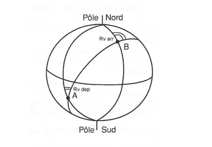
This difference appears clearly in this diagram. The value of this convergence can be evaluated using the following formula:
Conv = ∆ G x sin Lm
In this formula, delta G represents the difference in longitude between A and B, and Lm is the average of their latitudes.
We immediately see that if the longitude difference is small, the convergence will be very weak (or even zero on a meridian as already seen). On the other hand, it will be maximum for an East/West journey or vice versa.
Likewise, if the mean latitude is low, so will the convergence. So in equatorial regions, the great circle will practically be a rhumb line and vice versa!
So we can deduce from this formula that the convergence will be significant for great circle road segments at a fairly high mean latitude and with a significant longitude difference.
Givry fix
The Rv of the rhumb line, constant by definition, connecting these same two points will be, as a first approximation, the average of the two true departure and arrival routes of the corresponding ortho. The difference of the Rv loxo with the Rv departure of the ortho will therefore be half of the convergence.
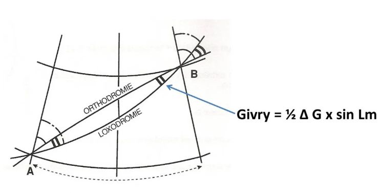
This value, also called Givry correction, named after the hydrographic engineer who created it, allows, for example, to trace the outline of a great circle on a Mercator map.
Nickname Givry
In the same way, there is a “pseudo-frost” which makes it possible to evaluate, on a Lambert map, the difference between the orthodromy and the straight map line.
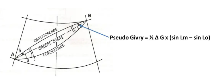
This formula, a little complicated I agree, above all allows us to show that if the road is located near the parallel of tangency Lo, the difference in the sines is practically zero, and therefore the pseudo-frost too, which allows us to say that the right map is practically a great circle.
The tangency parallel of a Lambert map, or the standard parallels of a secant Lambert map, will be chosen such that, in the region represented, the map is practically orthodromic.
The elements of a rhumb line, Rv and distance, while easy to measure on a Mercator map, are rather complicated to calculate with great precision. Conversely, orthodromy is not very simple to represent on a map with great precision and therefore to measure, but it is quite easy to calculate, thanks to spherical trigonometry in a position triangle, Rv departure and arrival and great circle distance. As it is also the most direct route, it is therefore not surprising that modern navigation computers make us follow great circles!
Application exercise
To finish and summarize all of this a little, I offer you a little application exercise.
You are taking a flight in the great Canadian North, which takes you along the east/west route which passes vertically over Resolute Bay. Here is represented, on a polar stereographic map, the segment of road on which you are located (click to enlarge).
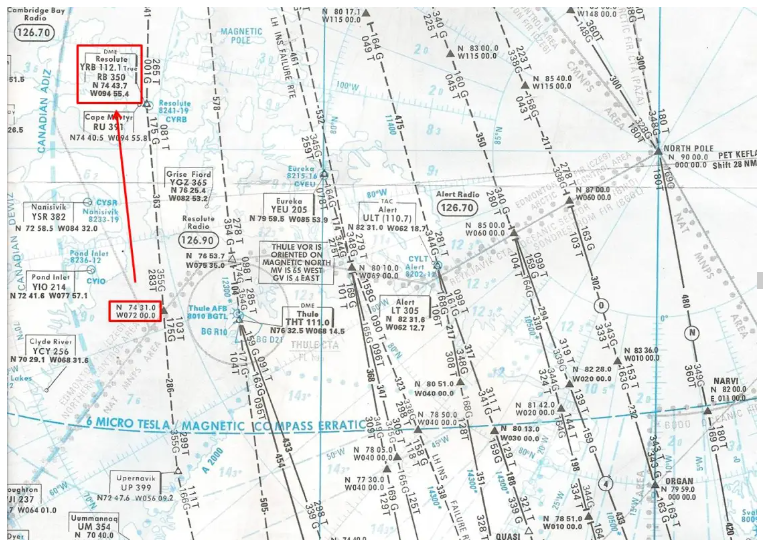
Yes, an East/West road represented by an almost vertical line is not very common!!! The polar stereographic map, you have to get used to it…
The convergence of the meridians is very important since, as seen on the map, on this segment, the departure Rv is 283° (283T) and the route Rv arriving at Resolute Bay is 261° (inverse of 081T indicated as Rv departure in the opposite direction). No less than 22°, a result that could also be verified by calculation by multiplying the difference in longitude, approximately 23°, by the sine of the mean latitude, approximately 75°.
In this polar region where the horizontal component of the Earth's magnetic field is very weak, less than 6 microteslas, you have set your compasses to true North.
You have passed the point N74°31.0 W072°00.0 for quite a while, and shortly after crossing the 080W you start to receive the VORDME from Resolute Bay, YBR. This one is set, like the other Canadian VORs located in the 6 microteslas zone, to true North (True indicated next to the frequency).
- You are reading a QUJ, true equivalent of the QDM of 261° (or true radial 081° in approximation). Are you on the planned route?
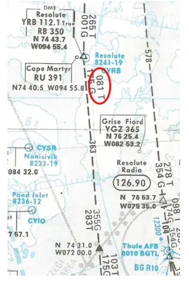
Yes, since the starting Rv of this segment, taken in reverse, is 081T as indicated on the map. The VOR radio waves move in a straight line, the plane is indeed on the great circle which has Rv arriving at YBR 261°.
At this point, you decide to guide the aircraft with the Hdg Sel function. The wind is zero.
- If you display heading 261°, will you follow the true radial 081° inbound? To follow it, would you need a stronger or weaker heading?
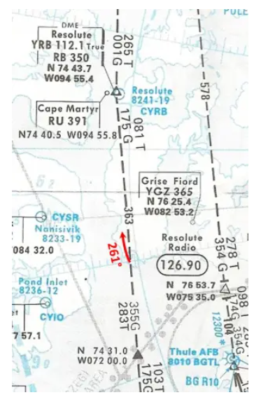
No. If we keep the true heading 261° constant, the plane will go south of the route. To follow the planned route, we would have to take a stronger course…
- At the time you switched to Hdg Sel, the Cv was 272°. If you stay this way will you fly over Resolute Bay? If not, what will need to be done?
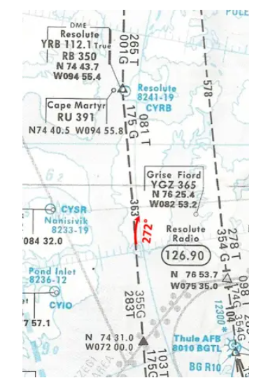
No. We will not fly over Resolute Bay because, by maintaining a constant heading of 272°, the plane will go north of the route. To follow the radial, it would be necessary to gradually decrease the heading to arrive at 261° at YRB.
- If, from the previous point N74°31.0 W072°00.0 you wanted to go to Resolute Bay at constant Rv, what heading should you have displayed (no wind)?
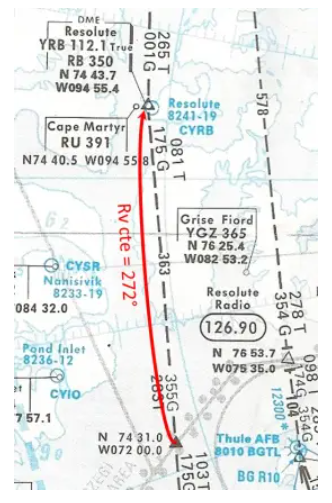
The constant RV will be the average of the departure RV and arrival RV:
(283 261)/2 = 272°
We find the same result by applying the Givry correction to the departure Rv:
g = ½(23 x sin 75°) = 11°
Rv cte = 283 – 11 = 272°
CHOOSE A ROUTE
It now remains to choose between orthodromy or rhumb line. As we have already seen, this choice will only have a certain importance over a long journey, and even more so if the east/west trend is significant.
So how to do it? For operators of airliners, which are very fuel-hungry, the ideal route is what is called the RTM for Minimum Time Route.
Without wind, RTM is great circle. But it is illusory to hope to make a long flight without experiencing the slightest wind...
There is a graphical method to find, based on the forecast winds, what the RTM would be. This is what was done in the past, by hand, it was the job of operations agents or other dispatchers.
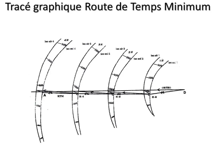
Today, they have software whose computing power makes it possible to evaluate all possible routes in a few moments...
Unfortunately, we do not have this type of tool for our simulated flights, but certain software gives a fairly similar and very acceptable result.
All this will be covered in the articles to follow…
CONCLUSION
This first part of the study of navigation sets the foundations which will allow us to better understand how navigation is practiced on a long-haul flight.
In the next articles, we will study the different means of navigation, how flight plans are developed and how a long-haul flight takes place.
Enjoy the flights everyone.